Machine Learning and Predictive Models
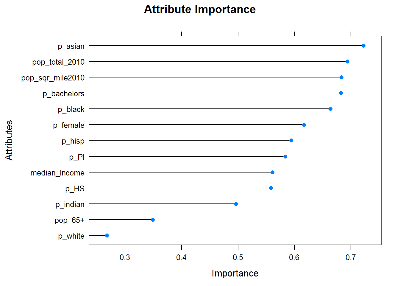
Variable Importance, 2012
Let’s take a look at variable importance with regards to US Census data (per-county basis) for 2012. Note the high importance of the attribute measuring the proportion of the county that was considered ‘Asian.’
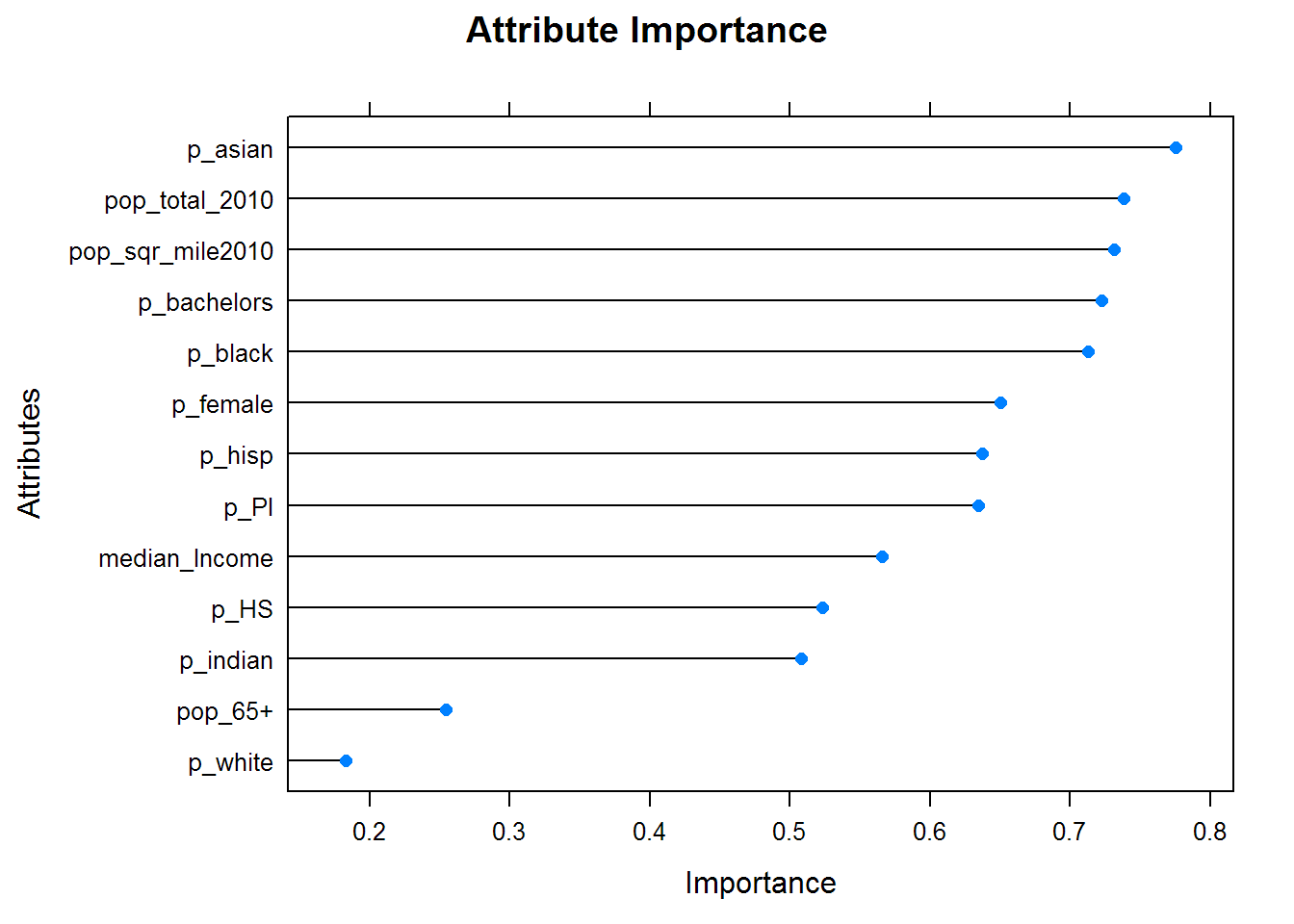
Variable Importance, 2016
We can perform the same importance analysis for 2016.
Conditional Inference Tree
We can build a conditional inference machine learning model to predict county-level outcomes on the 2012 data. In this case, our accuracy was 86.4% on our test data set (separated from training data). As a note, accuracy is measured by summing the top-left cell and the bottom-right cell (along the lower-right diagonal).
##
##
##    Cell Contents
## |-------------------------|
## |                       N |
## |         N / Table Total |
## |-------------------------|
##
##
## Total Observations in Table:  624
##
##
##              | Predicted Type
##  Actual Type |         0 |         1 | Row Total |
## -------------|-----------|-----------|-----------|
##            0 |       460 |        16 |       476 |
##              |     0.737 |     0.026 |           |
## -------------|-----------|-----------|-----------|
##            1 |        69 |        79 |       148 |
##              |     0.111 |     0.127 |           |
## -------------|-----------|-----------|-----------|
## Column Total |       529 |        95 |       624 |
## -------------|-----------|-----------|-----------|
##
##
We can use this model on 2016 data as well. Here, our accuracy decreased on testing data to 71.65%.
##
##
##    Cell Contents
## |-------------------------|
## |                       N |
## |         N / Table Total |
## |-------------------------|
##
##
## Total Observations in Table:  624
##
##
##                 | Predicted Type
##     Actual Type |         0 |         1 | Row Total |
## ----------------|-----------|-----------|-----------|
##    Donald Trump |       437 |        85 |       522 |
##                 |     0.700 |     0.136 |           |
## ----------------|-----------|-----------|-----------|
## Hillary Clinton |        92 |        10 |       102 |
##                 |     0.147 |     0.016 |           |
## ----------------|-----------|-----------|-----------|
##    Column Total |       529 |        95 |       624 |
## ----------------|-----------|-----------|-----------|
##
##
Sequential Covering and Rule-based Learning
We used a rule-based method (jRip) to model the 2012 data. Here, our accuracy in predicting county-level outcomes was 85.3%. We’ve also listed the rules below. Our successes with rule-based sequential covering methods (compared to conditional inference trees) suggests a lower level of complexity with regards to individual voting decisions.
For reference, the general syntax for the classification rules is: rule-set => prediction (# of instances correctly classified by rule, # of instances misclassified by rule).
## JRIP rules:
## ===========
##
## (p_white <= 53.5) and (p_hisp <= 29.3) and (p_black >= 46.6) => ObamaWin=1 (88.0/1.0)
## (p_asian >= 1.3) and (pop_sqr_mile2010 >= 446.7) and (p_white <= 68.6) => ObamaWin=1 (106.0/18.0)
## (p_asian >= 1.1) and (pop_sqr_mile2010 >= 282.7) and (p_female >= 51.4) => ObamaWin=1 (56.0/18.0)
## (p_bachelors >= 25.4) and (p_asian >= 3.4) and (pop_65+ >= 13.9) => ObamaWin=1 (36.0/8.0)
## (p_bachelors >= 28) and (p_hisp <= 2.2) => ObamaWin=1 (33.0/12.0)
## (p_asian >= 0.9) and (p_white <= 54.9) and (p_bachelors >= 15.9) => ObamaWin=1 (47.0/13.0)
## (p_bachelors >= 28) and (p_bachelors >= 39.4) and (pop_total_2010 <= 23509) => ObamaWin=1 (16.0/2.0)
## (p_white <= 31.5) => ObamaWin=1 (33.0/7.0)
##  => ObamaWin=0 (2074.0/209.0)
##
## Number of Rules : 9
##
##
## Cell Contents
## |-------------------------|
## | N |
## | N / Table Total |
## |-------------------------|
##
##
## Total Observations in Table: 624
##
##
## | Predicted Type
## Actual Type | 0 | 1 | Row Total |
## -------------|-----------|-----------|-----------|
## 0 | 448 | 28 | 476 |
## | 0.718 | 0.045 | |
## -------------|-----------|-----------|-----------|
## 1 | 64 | 84 | 148 |
## | 0.103 | 0.135 | |
## -------------|-----------|-----------|-----------|
## Column Total | 512 | 112 | 624 |
## -------------|-----------|-----------|-----------|
##
## Interestingly, when we apply this model trained on 2012 data to the 2016 data, our accuracy on test data increases to 93.5% (or in other words, we are able to correctly predict county-level outcomes 93.5% of the time)
##
##
##    Cell Contents
## |-------------------------|
## |                       N |
## |         N / Table Total |
## |-------------------------|
##
##
## Total Observations in Table:  624
##
##
##                 | Predicted Type
##     Actual Type |         0 |         1 | Row Total |
## ----------------|-----------|-----------|-----------|
##    Donald Trump |       504 |        18 |       522 |
##                 |     0.808 |     0.029 |           |
## ----------------|-----------|-----------|-----------|
## Hillary Clinton |        23 |        79 |       102 |
##                 |     0.037 |     0.127 |           |
## ----------------|-----------|-----------|-----------|
##    Column Total |       527 |        97 |       624 |
## ----------------|-----------|-----------|-----------|
##
##
## JRIP rules:
## ===========
##
## (p_white <= 47.1) and (p_indian <= 1) => lead=Hillary Clinton (132.0/15.0)
## (p_bachelors >= 27.3) and (p_asian >= 3.5) => lead=Hillary Clinton (135.0/36.0)
## (p_white <= 54.9) and (pop_sqr_mile2010 >= 48.9) and (pop_sqr_mile2010 >= 303.8) => lead=Hillary Clinton (18.0/0.0)
## (p_white <= 54.1) and (p_white <= 33.3) and (p_white <= 23.3) => lead=Hillary Clinton (15.0/1.0)
## (p_bachelors >= 25.6) and (pop_sqr_mile2010 >= 619.7) and (pop_sqr_mile2010 >= 1115.3) => lead=Hillary Clinton (19.0/4.0)
## (p_bachelors >= 28) and (p_bachelors >= 39.4) => lead=Hillary Clinton (32.0/11.0)
## (p_bachelors >= 27.3) and (p_hisp <= 2.2) and (p_black <= 0.7) => lead=Hillary Clinton (14.0/4.0)
## (p_white <= 54.9) and (pop_sqr_mile2010 >= 48.9) and (median_Income <= 34285) => lead=Hillary Clinton (9.0/0.0)
## (p_bachelors >= 21.3) and (p_hisp >= 23.5) and (p_indian >= 2.1) and (pop_sqr_mile2010 >= 4.7) => lead=Hillary Clinton (10.0/0.0)
## (p_white <= 52.3) and (p_hisp <= 10.1) and (median_Income >= 36022) and (pop_total_2010 >= 7065) => lead=Hillary Clinton (12.0/3.0)
## (p_bachelors >= 18.2) and (p_white <= 36) => lead=Hillary Clinton (6.0/0.0)
## => lead=Donald Trump (2087.0/57.0)
##
## Number of Rules : 12If we train a model and test it with purely 2016 data, interestingly, our accuracy decreases to 92%.
##
##
##    Cell Contents
## |-------------------------|
## |                       N |
## |         N / Table Total |
## |-------------------------|
##
##
## Total Observations in Table:  624
##
##
##                 | Predicted Type
##     Actual Type |    Donald Trump | Hillary Clinton |       Row Total |
## ----------------|-----------------|-----------------|-----------------|
##    Donald Trump |             498 |              24 |             522 |
##                 |           0.798 |           0.038 |                 |
## ----------------|-----------------|-----------------|-----------------|
## Hillary Clinton |              26 |              76 |             102 |
##                 |           0.042 |           0.122 |                 |
## ----------------|-----------------|-----------------|-----------------|
##    Column Total |             524 |             100 |             624 |
## ----------------|-----------------|-----------------|-----------------|
##
##
kNN
We also used a k-nearest-neighbor algorithm for 2012 and 2016 data. With 2012 data, we were able to achieve an accuracy of 86.8%.
##
##
##    Cell Contents
## |-------------------------|
## |                       N |
## |           N / Row Total |
## |           N / Col Total |
## |         N / Table Total |
## |-------------------------|
##
##
## Total Observations in Table:  623
##
##
##                 | prc_test_pred
## prc_test_labels |         0 |         1 | Row Total |
## ----------------|-----------|-----------|-----------|
##               0 |       465 |        11 |       476 |
##                 |     0.977 |     0.023 |     0.764 |
##                 |     0.868 |     0.126 |           |
##                 |     0.746 |     0.018 |           |
## ----------------|-----------|-----------|-----------|
##               1 |        71 |        76 |       147 |
##                 |     0.483 |     0.517 |     0.236 |
##                 |     0.132 |     0.874 |           |
##                 |     0.114 |     0.122 |           |
## ----------------|-----------|-----------|-----------|
##    Column Total |       536 |        87 |       623 |
##                 |     0.860 |     0.140 |           |
## ----------------|-----------|-----------|-----------|
##
##
Using 2016 training and testing data, our accuracy on a county-level basis increased to 93.57%.
##
##
##    Cell Contents
## |-------------------------|
## |                       N |
## |           N / Row Total |
## |           N / Col Total |
## |         N / Table Total |
## |-------------------------|
##
##
## Total Observations in Table:  623
##
##
##                 | prc_test_pred
## prc_test_labels |    Donald Trump | Hillary Clinton |       Row Total |
## ----------------|-----------------|-----------------|-----------------|
##    Donald Trump |             506 |              15 |             521 |
##                 |           0.971 |           0.029 |           0.836 |
##                 |           0.953 |           0.163 |                 |
##                 |           0.812 |           0.024 |                 |
## ----------------|-----------------|-----------------|-----------------|
## Hillary Clinton |              25 |              77 |             102 |
##                 |           0.245 |           0.755 |           0.164 |
##                 |           0.047 |           0.837 |                 |
##                 |           0.040 |           0.124 |                 |
## ----------------|-----------------|-----------------|-----------------|
##    Column Total |             531 |              92 |             623 |
##                 |           0.852 |           0.148 |                 |
## ----------------|-----------------|-----------------|-----------------|
##
##
Prediction Mapping
We can use our jRip model on all of the 2016 data, not just the test data, with an accuracy of 93% (note the potential for bias due to the fact that the training data is being recycled for the prediction).
## JRIP rules:
## ===========
##
## (p_white <= 52.3) and (p_hisp <= 28) => ObamaWin=1 (230.0/31.0)
## (p_asian >= 1.3) and (pop_total_2010 >= 266929) and (pop_total_2010 >= 735332) => ObamaWin=1 (54.0/6.0)
## (p_asian >= 1.3) and (p_bachelors >= 27.7) and (pop_65+ >= 13.5) and (p_asian >= 2.7) => ObamaWin=1 (69.0/18.0)
## (p_bachelors >= 25.1) and (p_bachelors >= 38.7) and (median_Income <= 72745) => ObamaWin=1 (64.0/18.0)
## (p_asian >= 1.1) and (pop_sqr_mile2010 >= 492.6) and (p_HS <= 88.8) and (pop_sqr_mile2010 >= 1115.3) => ObamaWin=1 (16.0/2.0)
## (p_asian >= 1.1) and (pop_total_2010 >= 153920) and (p_white <= 59.5) => ObamaWin=1 (33.0/12.0)
## (p_white <= 55.7) and (p_white <= 32) => ObamaWin=1 (33.0/7.0)
## (p_HS >= 86.5) and (pop_sqr_mile2010 >= 16.6) and (p_HS >= 89.6) and (p_hisp <= 2.2) and (p_asian >= 0.6) and (median_Income <= 57565) and (p_bachelors >= 25.9) and (pop_sqr_mile2010 <= 199) => ObamaWin=1 (22.0/1.0)
##  => ObamaWin=0 (2591.0/266.0)
##
## Number of Rules : 9
##
##
## Cell Contents
## |-------------------------|
## | N |
## | N / Table Total |
## |-------------------------|
##
##
## Total Observations in Table: 3112
##
##
## | Predicted Type
## Actual Type | 0 | 1 | Row Total |
## ----------------|-----------|-----------|-----------|
## Donald Trump | 2500 | 125 | 2625 |
## | 0.803 | 0.040 | |
## ----------------|-----------|-----------|-----------|
## Hillary Clinton | 91 | 396 | 487 |
## | 0.029 | 0.127 | |
## ----------------|-----------|-----------|-----------|
## Column Total | 2591 | 521 | 3112 |
## ----------------|-----------|-----------|-----------|
##
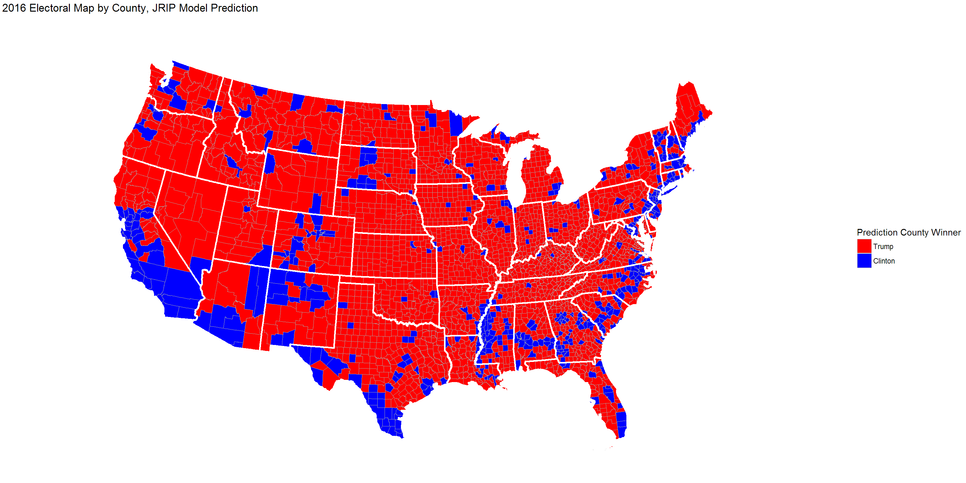
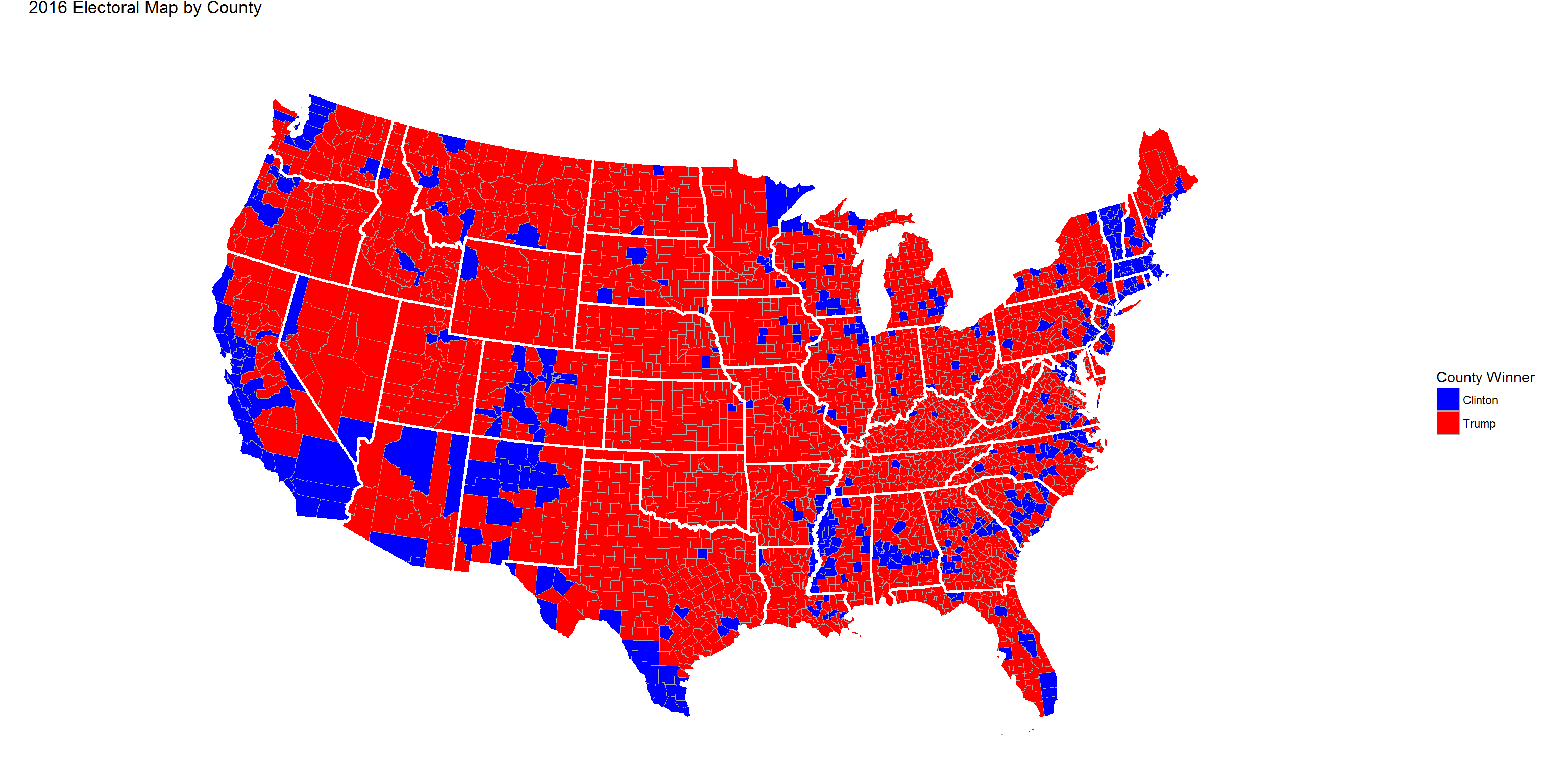
## 2016 Prediction Map
We can map the result of our jRip model and compare it to the actual 2016 result.
2016 Actual Map
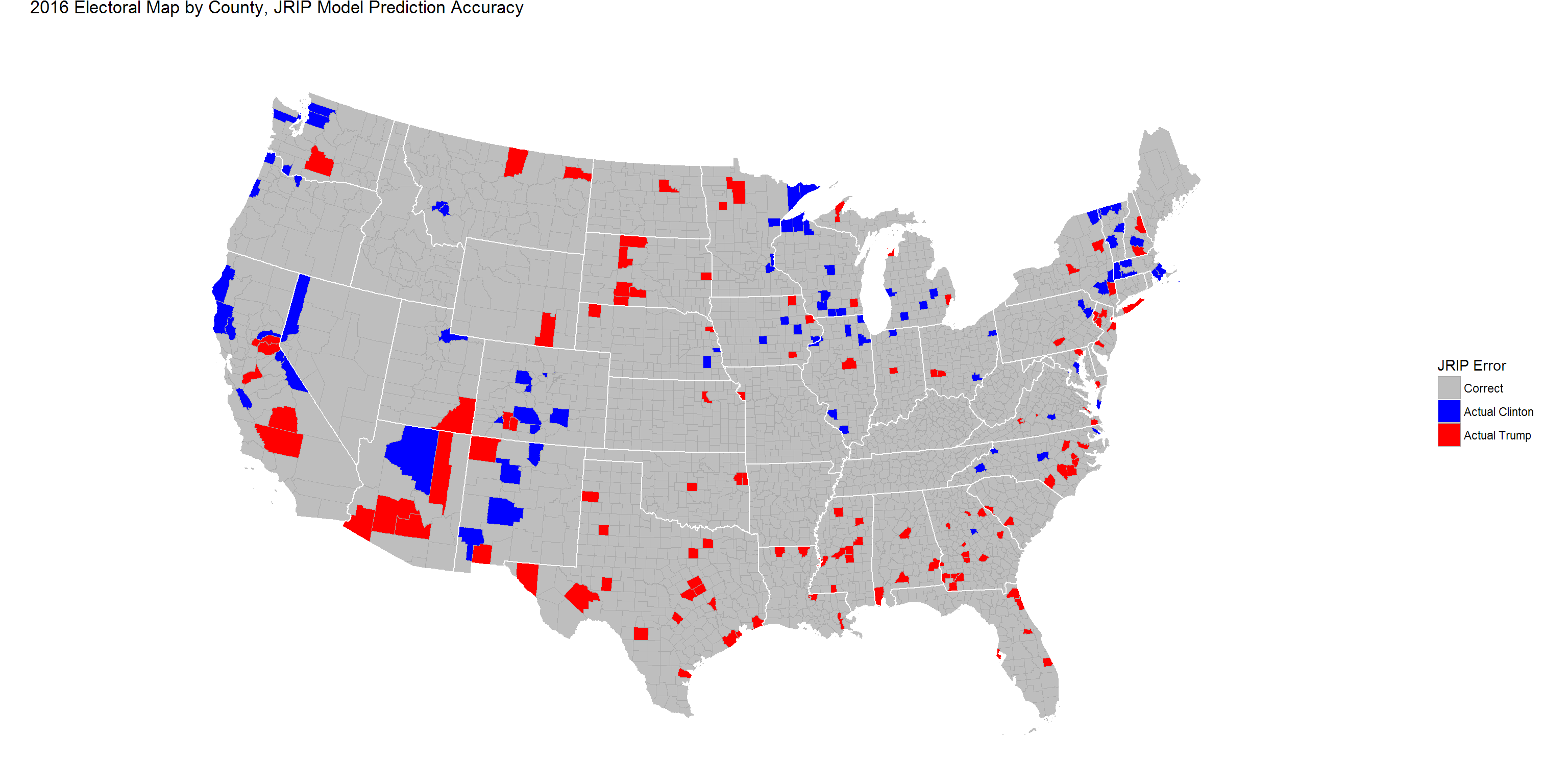
Prediction Error Visualized
We can actually visualize our model’s prediction error. The counties in grey represent correct predictions, while blue highlights represent Trump predictions that actually voted for Clinton and red highlights represent Clinton predictions that actually voted for Trump.
Additionally, while these models are able to predict county-level results on a win/loss basis, they are unable to predict Clinton/Trump votes in the area.